


Introduction
In this article, I will give you an introduction to the Naïve Bayes algorithm. It is simple but also a fast algorithm. It has been successfully used for many purposes, but it works well with natural language processing problems. It is a classification technique based on Bayes’ Theorem. It assumes that a particular feature in a class is not related to the presence of other features. But those assumptions(that the features are independent) might not always be true when implemented over a real-world dataset. That’s why this classifier has the term ‘Naive’ in its name.
Here’s the Bayes theorem, which is the basic for this algorithm:
Let's take a look at Bayes theorem.
Bayes’ Theorem finds the probability of an event occurring given the probability of another event that has already occurred. Bayes’ theorem is stated mathematically as the following equation:
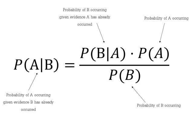 Where A and B are events and P(B)≠0
P(A|B) is a conditional probability: the likelihood of event A occurring given that B is true.
P(B|A) is also a conditional probability: the likelihood of event B occurring given that A is true.
P(A) and P(B) are the probabilities of observing A and B respectively; they are known as the marginal probability.
Algorithm steps:
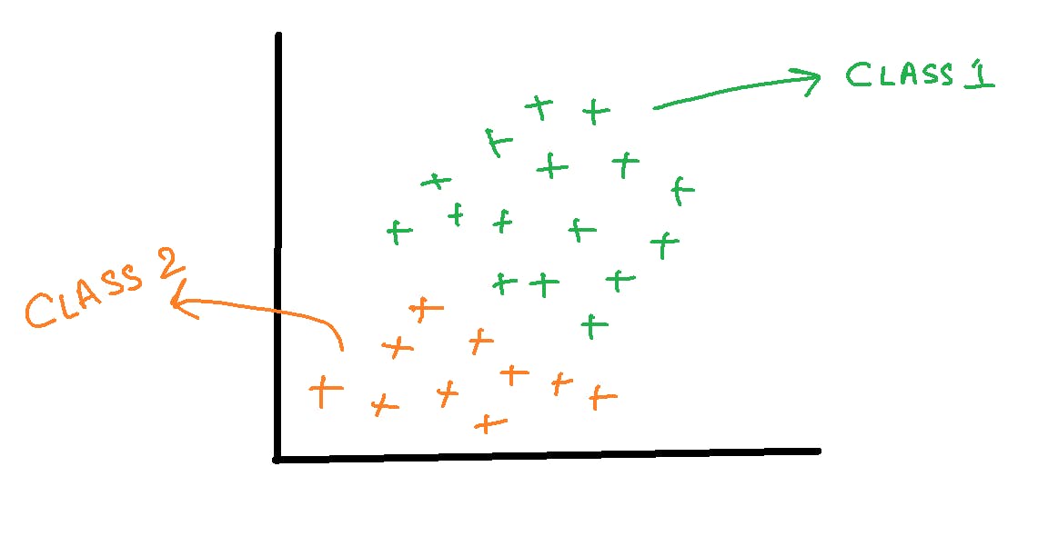
1.Let’s consider that we have a binary classification problem i.e., we have two classes in our data as shown below.
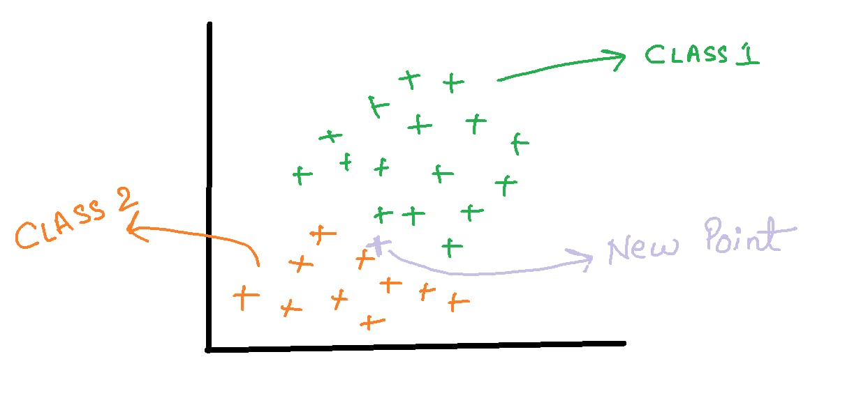
- Now suppose if we are given a new data point, to which class does that point belong to?
- The formula for a point ‘X’ to belong in class1 can be written as: Where the numbers represent the order in which we are going to calculate different probabilities.
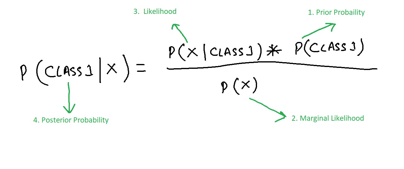
A similar formula can be utilized for class 2 as well.
Probability of class 1 can be written as: P(class1)=Number of points in class1/Total number of points= 16/26=0.62
For calculating the probability of X, we draw a circle around the new point and see how many points(excluding the new point) lie inside that circle. The points inside the circle are considered to be similar points.
P(X)=Number of similar observation/Total Observations=3/26=0.12
Now, we need to calculate the probability of a point to be in the circle that we have made given that it’s of class 1. P(X | Class1)= Number of points in class 1 inside the circle/Total number of points in class 1=1/16=0.06
We can substitute all the values into the formula in step 3. We get: P(Class1 | X)=0.06*0.62/0.12=0.31
And if we calculate the probability that X belongs to Class2, we’ll get 0.69. It means that our point belongs to class 2.
The Generalization for Multiclass:
The approach discussed above can be generalized for multiclass problems as well. Suppose, P1, P2, P3…Pn is the probabilities for the classes C1, C2, C3…Cn, then the point X will belong to the class for which the probability is maximum. Or mathematically the point belongs to the result of argmax(P1,P2,P3….Pn)
Pros and Cons of Naive Bayes?
Pros:
It is easy and fast to predict test data set.
It also performs well in multi-class prediction
Naive Bayes classifier performs better compared to other models like logistic regression and you need less training data.
It performs well in the case of categorical input variables compared to the numerical variables.
Cons:
If a categorical variable has a category (in the test data set), which was not observed in the training data set, then the model will assign a 0 (zero) probability and will be unable to make a prediction. This is often known as “Zero Frequency”. To solve this, we can use Laplace estimation.
On the other side Naive Bayes is also known as a bad estimator, so the probability outputs from predict_proba are not to be taken too seriously.
Another limitation of Naive Bayes is the assumption of independent predictors. In real life, it is almost impossible that we get a set of predictors that are completely independent.